I frequently use KDE plots for my work, but I have not previously used them for spatial analysis. I found a really cool example here using the geoplot Python library. geoplot uses Seaborn behind the scenes to generate the KDE plots.

Unfortunately, geoplot didn’t work for me and I set about finding my own solution. In this post, I explain how I acheived that.

Data: fatal crashes in Brisbane

I will work with the vehicle crashes dataset from Queensland roads, which is available from the Queensland open data portal. This dataset provides information on location and characteristics of crashes in Queensland for all reported road traffic crashes that occurred from 1 January 2001 to 30 November 2023.

I only want to focus on fatal crashes, so the only three columns of interest are Crash_Longitude, Crash_Latitutde, and Count_Casualty_Fatality. And of course only those with a fatality (Count_Casualty_Fatality > 0).

import pandas as pd

fatal_crashes = pd.read_csv(
    '../data/qld-road-crash-locations.csv',
    usecols=['Crash_Longitude', 'Crash_Latitude', 'Count_Casualty_Fatality'],
)
fatal_crashes = fatal_crashes[fatal_crashes['Count_Casualty_Fatality'] > 0]

The above data is still for all of QLD, so the next step is to get Brisbane’s council boundaries and retain only those crashes that happened within the council boundaries. I will use a GeoParquet file for this (shared on GitHub here).

import geopandas as gpd

# dissolve because we only need the outer boundaries
brisbane = gpd.read_parquet('../data/brisbane-suburbs.parq').dissolve()

# convert to a geodataframe
fatal_crashes = gpd.GeoDataFrame(
    fatal_crashes,
    geometry=gpd.points_from_xy(fatal_crashes['Crash_Longitude'], fatal_crashes['Crash_Latitude']),
    crs=brisbane.crs
).drop(columns=['Crash_Longitude', 'Crash_Latitude']).clip(brisbane)

fatal_crashes.head()

	Count_Casualty_Fatality	geometry
362708	1	POINT (153.00744 -27.6564)
388774	1	POINT (153.00476 -27.65595)
120572	1	POINT (153.00375 -27.6558)
210495	1	POINT (152.99434 -27.65306)
267168	1	POINT (152.96758 -27.63583)

First attempt with geoplot

When I used the geoplot example (here), I got an error 'MultiPolygon' object is not iterable, which is most likely caused by API changes to either Seaborn, Matplotlib because geoplot was last updated 2 years ago. Perhaps its also related to this open issue.

import geoplot as gplt
import matplotlib.pyplot as plt
import contextily as cx

fig, ax = plt.subplots()

gplt.kdeplot(
    fatal_crashes,
    cmap='viridis',
    thresh=0.05,
    clip=brisbane.geometry,
    ax=ax
)
gplt.polyplot(brisbane, zorder=1, ax=ax)

---------------------------------------------------------------------------
TypeError                                 Traceback (most recent call last)
File ~/data-science/.venv/lib/python3.12/site-packages/geoplot/geoplot.py:885, in polyplot.<locals>.PolyPlot.draw(self)
    884 try:  # Duck test for MultiPolygon.
--> 885     for subgeom in geom:
    886         feature = GeopandasPolygonPatch(
    887             subgeom, facecolor=facecolor, edgecolor=edgecolor, zorder=zorder,
    888             **kwargs
    889         )

TypeError: 'MultiPolygon' object is not iterable

During handling of the above exception, another exception occurred:

AttributeError                            Traceback (most recent call last)
Cell In[19], line 14
      5 fig, ax = plt.subplots()
      7 gplt.kdeplot(
      8     fatal_crashes,
      9     cmap='viridis',
   (...)     12     ax=ax
     13 )
---> 14 gplt.polyplot(brisbane, zorder=1, ax=ax)

File ~/data-science/.venv/lib/python3.12/site-packages/geoplot/geoplot.py:901, in polyplot(df, projection, extent, figsize, ax, **kwargs)
    898         return ax
    900 plot = PolyPlot(df, figsize=figsize, ax=ax, extent=extent, projection=projection, **kwargs)
--> 901 return plot.draw()

File ~/data-science/.venv/lib/python3.12/site-packages/geoplot/geoplot.py:892, in polyplot.<locals>.PolyPlot.draw(self)
    890                 ax.add_patch(feature)
    891         except (TypeError, AssertionError):  # Shapely Polygon.
--> 892             feature = GeopandasPolygonPatch(
    893                 geom, facecolor=facecolor, edgecolor=edgecolor, zorder=zorder,
    894                 **kwargs
    895             )
    896             ax.add_patch(feature)
    898 return ax

File ~/data-science/.venv/lib/python3.12/site-packages/geopandas/plotting.py:108, in _PolygonPatch(polygon, **kwargs)
    104 from matplotlib.patches import PathPatch
    105 from matplotlib.path import Path
    107 path = Path.make_compound_path(
--> 108     Path(np.asarray(polygon.exterior.coords)[:, :2]),
    109     *[Path(np.asarray(ring.coords)[:, :2]) for ring in polygon.interiors],
    110 )
    111 return PathPatch(path, **kwargs)

AttributeError: 'MultiPolygon' object has no attribute 'exterior'

Initial KDE plot

So, I set about finding my own solution, and that’s when I came across this post by Håvard Wallin Aagesen that shows how to use Seaborn’s kdeplot for geospatial analysis. I have used that as an inspiration to generate a plot similar to that in the geoplot example.

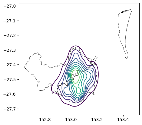
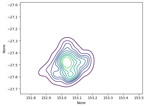
The first step is drawing the KDE plot using Seaborn. We can see in the plot below that seaborn has drawn 10 contours by default.

import matplotlib.pyplot as plt
import seaborn as sns

fig, ax = plt.subplots()
brisbane.boundary.plot(ax=ax, edgecolor='black', linewidth=0.5)
sns.kdeplot(fatal_crashes, x=fatal_crashes.geometry.x, y=fatal_crashes.geometry.y, weights='Count_Casualty_Fatality', cmap='viridis', ax=ax)
ax.set(xlabel='', ylabel='')
plt.show()

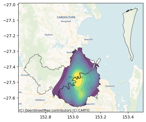
We can see that some of the contours extend beyond the city’s boundaries, but in the reference example from geoplot, the contours are within the city limit, and that’s what I want to achieve.

The solution is to individually access these contours, convert them into Polygons (or MultiPolygons), and then trim them using the city boundaries. Credit goes to this Medium article for the initial idea. Some of the example code in that article didn’t work for me (perhaps due to upstream changes with seaborn?).

Improved KDE plot clipped to boundaries

Getting individual contour regions

Seaborn’s kdeplot returns a collection of children, including a QuadContourSet instance that contains information about the contour and contour regions.

kde = sns.kdeplot(fatal_crashes, x=fatal_crashes.geometry.x, y=fatal_crashes.geometry.y, weights='Count_Casualty_Fatality', cmap='viridis')

import pprint

pprint.pp(kde.get_children())

[<matplotlib.contour.QuadContourSet object at 0x7fe103723800>,
 <matplotlib.spines.Spine object at 0x7fe10353c920>,
 <matplotlib.spines.Spine object at 0x7fe10353e750>,
 <matplotlib.spines.Spine object at 0x7fe10357ea80>,
 <matplotlib.spines.Spine object at 0x7fe10357ee70>,
 <matplotlib.axis.XAxis object at 0x7fe103a38500>,
 <matplotlib.axis.YAxis object at 0x7fe10357f080>,
 Text(0.5, 1.0, ''),
 Text(0.0, 1.0, ''),
 Text(1.0, 1.0, ''),
 <matplotlib.patches.Rectangle object at 0x7fe103723f20>]

Clipping contour regions to boundaries

And each QuadCountourSet instance is a collection of contour paths, which we can access with the get_paths method. We can generate a shapely Polygon using the to_polygons method.

# credit to https://towardsdatascience.com/from-kernel-density-estimation-to-spatial-analysis-in-python-64ddcdb6bc9b/

from shapely import Polygon
from matplotlib.contour import QuadContourSet

contour_set = None
for i in kde.get_children():
    if type(i) is QuadContourSet:
        contour_set = i
        break

contour_paths = []
# Loop through all contours
for contour in contour_set.get_paths(): 
    # Create a polygon for the countour
    # First polygon is the main countour, the rest are holes
    for ncp,cp in enumerate(contour.to_polygons()):
        x = cp[:,0]
        y = cp[:,1]
        new_shape = Polygon([(i[0], i[1]) for i in zip(x,y)])
        if ncp == 0:
            poly = new_shape
        else:
            # Remove holes, if any
            poly = poly.difference(new_shape)

    # Append polygon to list
    contour_paths.append(poly)

# make holes corresponding to the inner contours
contour_polys = [contour_paths[i].difference(contour_paths[i+1]) for i in range(len(contour_paths)-2)] + [contour_paths[-1]]

df = pd.DataFrame(zip(contour_set.levels, contour_polys), columns=['level', 'geometry'])
gdf = gpd.GeoDataFrame(df, crs=brisbane.crs)

clipped_kde_gdf = gdf.clip(brisbane)

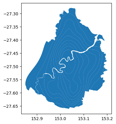
Now, if we plot clipped_kde_gdf, we can see that the contour has been nicely clipped to Brisbane’s boundaries.

clipped_kde_gdf.plot()

Final plot

Finally, we can plot the complete plot, this time with some background tiles.

import contextily as cx

fig, ax = plt.subplots()
brisbane.boundary.plot(ax=ax, edgecolor='black', linewidth=0.5)
cx.add_basemap(ax, crs=brisbane.crs, source=cx.providers.CartoDB.Voyager)
clipped_kde_gdf.plot('level', ax=ax, cmap='viridis', alpha=0.7)
ax.set(xlabel='', ylabel='')
plt.show()